The perceptron represents one of the most fundamental building blocks of modern artificial intelligence and deep learning. To truly understand what a perceptron is and why it matters, we need to journey back to 1943 and trace its evolution from the first computational model of a neuron to the sophisticated neural networks we use today.
The Biological Inspiration
Before diving into artificial neurons, let's understand what inspired them. The human brain contains approximately 100 billion neurons working in a massively parallel interconnected network. Each biological neuron has dendrites that receive signals from other neurons, a soma (cell body) that processes the incoming information, an axon that transmits the output signal to other neurons, and synapses as connection points where neurons communicate.
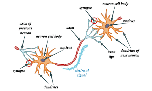
A neuron acts like a biological switch. It receives multiple input signals, processes them, and either "fires" (sends an output signal) or stays silent based on whether the combined input exceeds a certain threshold.
The McCulloch-Pitts Neuron (1943)
The First Mathematical Model
Warren McCulloch, a neuroscientist, and Walter Pitts, a logician, published their groundbreaking paper in 1943 attempting to understand how the brain produces complex patterns using interconnected basic cells. Their model, known as the McCulloch-Pitts (MCP) neuron, was humanity's first mathematical representation of a biological neuron.
How the McCulloch-Pitts Neuron Works
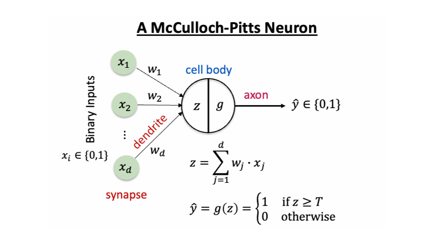
The MCP neuron operates in two distinct phases. First, in the aggregation phase, the neuron receives multiple binary inputs (either 0 or 1), where each input represents a signal from another neuron. These inputs can be either excitatory or inhibitory.
Second, in the threshold decision phase, the neuron sums all the excitatory inputs. If ANY inhibitory input is present, the neuron immediately outputs 0 (doesn't fire). Otherwise, if the sum of excitatory inputs meets or exceeds a predetermined threshold (θ), the neuron outputs 1 (fires). If the sum is below the threshold, the neuron outputs 0.
Sum = x₁ + x₂ + ... + xₙ

Output = {
  0, if any inhibitory input is present
  1, if Sum ≥ θ
  0, if Sum < θ
}
Example: Implementing Logic Gates
The elegance of the MCP model lies in its ability to implement Boolean logic operations. An AND Gate (threshold = 2) has two excitatory inputs and fires only when both inputs are 1. An OR Gate (threshold = 1) has two excitatory inputs and fires when at least one input is 1. A NOT Gate (threshold = 0) has one inhibitory input—when the input is 1, the neuron doesn't fire (output 0), and when the input is 0, the threshold is reached (output 1).
Key Limitations of McCulloch-Pitts
- No Learning Mechanism: Weights and thresholds are fixed from the start
- Binary Inputs/Outputs: Can only handle 0s and 1s, not continuous values
- Unweighted Inputs: All excitatory inputs contribute equally
- Fixed Architecture: Once designed, the network cannot adapt
- Simple Inhibition: Any inhibitory signal completely prevents firing
Despite these limitations, the McCulloch-Pitts model demonstrated that networks of such neurons are Turing complete and can support universal computation.
The Rosenblatt Perceptron (1958)
Evolution Beyond McCulloch-Pitts
Frank Rosenblatt, building on the McCulloch-Pitts neuron and Hebbian learning principles, developed the first perceptron with the crucial ability to learn through weight adjustment. Published in his 1962 book "Principles of Neurodynamics," the perceptron represented a major leap forward in artificial intelligence.
Key Innovations
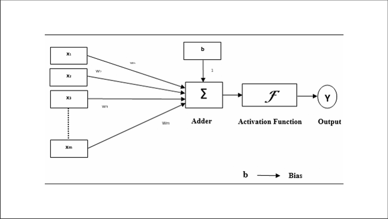
The Rosenblatt perceptron introduced several critical improvements: weighted inputs where each input has an associated weight, a learning algorithm where weights adjust based on training data, continuous weights that can be any real number (not just 0 or 1), a bias term as an adjustable threshold parameter, and real-valued inputs that can process continuous values rather than just binary.
Mathematical Formulation
The perceptron computes a weighted sum in the first step and then applies an activation function. The weighted sum is calculated as:
z = w₀ + w₁x₁ + w₂x₂ + ... + wₙxₙ

Or more compactly: z = w₀ + w·x
Then the activation function produces the output:
For binary classification:
y = {
  +1, if z ≥ 0
  -1, if z < 0
}
The Perceptron Learning Algorithm
The perceptron can learn from examples through an iterative process. First, initialize all weights to small random values (or zeros). Then, for each training example (x, target), compute the output ŷ = sign(w·x + w₀), calculate the error as error = target - ŷ, update weights using wᵢ = wᵢ + η × error × xᵢ, and update bias using w₀ = w₀ + η × error (where η is the learning rate, typically a small value like 0.1). Repeat this process until all examples are classified correctly or maximum iterations are reached.
Geometric Interpretation: Decision Boundaries
The perceptron creates decision boundaries that separate different classes of inputs in multidimensional space. For two-dimensional input (x₁, x₂), the decision boundary is represented by the equation:
Decision boundary: w₀ + w₁x₁ + w₂x₂ = 0
This equation represents a line (in 2D) or hyperplane (in higher dimensions) that divides the input space into two regions. Points above the line belong to Class +1, while points below the line belong to Class -1.
The XOR Problem: Understanding Perceptron Limitations
In 1969, Marvin Minsky and Seymour Papert proved a fundamental limitation: the perceptron could only solve linearly separable problems and could not solve XOR and NXOR functions. The XOR truth table shows that (0,0) → 0, (0,1) → 1, (1,0) → 1, and (1,1) → 0. No single straight line can separate the 1s from the 0s in this pattern, making it impossible for a single-layer perceptron to learn XOR. This limitation led to the "AI winter" until multi-layer networks were developed in the 1980s.
Comparing McCulloch-Pitts and Rosenblatt Perceptrons
| Feature | McCulloch-Pitts | Rosenblatt Perceptron |
|---|---|---|
| Year | 1943 | 1958 |
| Input Type | Binary (0 or 1) | Real-valued |
| Weights | Unweighted (or fixed) | Learnable real values |
| Learning | None | Perceptron learning algorithm |
| Threshold | Fixed | Adjustable (bias) |
| Purpose | Theoretical model | Practical pattern recognition |
The Perceptron as the Foundation of Neural Networks
Why Perceptrons Matter Today
While a single perceptron has limitations, it forms the fundamental unit of modern deep neural networks. Multi-Layer Perceptrons (MLPs) stack multiple layers of perceptrons to overcome the linear separability limitation. Modern activation functions replace the step function with smooth, differentiable functions like sigmoid, ReLU, and tanh. Backpropagation extends the perceptron learning principle to deep networks. With non-linear activations, MLPs gain universal approximation capability—they can approximate any continuous function.
From Perceptron to Deep Learning
The evolution continues from the McCulloch-Pitts neuron (1943) to the Rosenblatt Perceptron (1958), then to Multi-Layer Perceptrons (1980s), Deep Neural Networks (2006+), and finally to modern architectures like CNNs, RNNs, and Transformers that power today's AI revolution.
Practical Example: Binary Classification
Suppose we want to classify flowers as "Setosa" (+1) or "Not Setosa" (-1) based on petal length and width. Given training data like (1.4, 0.2) → +1 for Setosa and (4.5, 1.5) → -1 for Not Setosa, the perceptron learning process begins by initializing weights to zero with a learning rate of 0.1.
For the first example (1.4, 0.2) with target +1, we compute z = 0, so ŷ = +1, error = 0, and no update is needed. We continue with other examples, adjusting weights when predictions are wrong. After several epochs, the perceptron learns a decision boundary that successfully separates the classes.
Key Takeaways
- The McCulloch-Pitts neuron provided the first mathematical model of neural computation
- It demonstrated that simple neuron-like units could perform logical operations
- The Rosenblatt perceptron added the crucial ability to learn from data
- Single perceptrons are limited to linearly separable problems
- Modern neural networks extend these principles into powerful learning systems
The journey from McCulloch-Pitts neurons to modern perceptrons illustrates a fundamental principle in AI: simple computational units, when combined with learning mechanisms and proper architecture, can solve complex problems. Understanding these foundational concepts is essential for anyone working with machine learning and deep learning today, as they form the conceptual building blocks of even the most sophisticated AI systems.
Further Reading
- McCulloch, W.S., & Pitts, W. (1943). "A logical calculus of the ideas immanent in nervous activity"
- Rosenblatt, F. (1962). "Principles of Neurodynamics: Perceptrons and the Theory of Brain Mechanisms"
- Minsky, M., & Papert, S. (1969). "Perceptrons: An Introduction to Computational Geometry"